German pension mode
See also Present Values: Benefits payable (m)thly – pension modes other than German.
In the German pension mode, the present value of annuities is determined precisely if payments are made annually and for all payments made during a certain period, regardless of payment frequency. If annuity payments are made more frequently than annually, however, the life contingent payments in each year are discounted to the beginning of the payment year, according to the Richttafeln methodology. The factor ProVal uses to discount to the beginning of the payment year is displayed in the (active and inactive) sample life output under the payment frequency adjustment column(s).
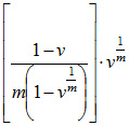
Generally, for beginning-of-period payment timing, for an annuity benefit payable (m)thly over the year to a life aged x, the factor is:
![]() for the life-contingent payments, and
for the life-contingent payments, and
 for the certain period payments
where:
![]() is the number of payments per year
is the number of payments per year
![]() if using RT 1998, 2005, or 2018, and
if using RT 1998, 2005, or 2018, and
 if using RT 1983
![]() is the interest discount factor for one year at annual interest rate i
is the interest discount factor for one year at annual interest rate i
![]() is the probability that the participant survives from age x to age x+1.
is the probability that the participant survives from age x to age x+1.
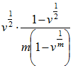
Likewise, for end-of-period payment timing, for an annuity benefit payable (m)thly over the year to a life aged x, the factor generally is:
![]() for the life-contingent payments, and
for the life-contingent payments, and
 for the certain period payments.
Note that end-of-period timing is always assumed for life insurance forms of payment.
The benefit payment frequency (m) applies only to annuities and life insurance (not to lump sum payment forms) and is specified under the Plan Attributes topic of the Plan Definition. (Note: if the “Continuous” option is selected, m is set equal to 10 million for a certain only annuity and to 10 million squared for any other type of annuity – that is, 10 raised to the seventh power and 10 raised to the 14th power, respectively.)
The payment frequency adjustments do not apply when payments are made annually (i.e., when m=1).
If using RT 1998, 2005, or 2018, the payment frequency adjustments above apply to all payment years except for the year of decrement from active status, when the contingency initiating the benefit is disability or death. Under those latter formulae, the mid-year commencement of disability and death decrements is reflected in the payment form value by means of the payment frequency adjustment in that year. If using the RT 1983 formulae, the payment frequency adjustments above apply to all payment years without exception. Under that method, mid-year commencement of death and disability benefits is reflected via averaging of annuity amounts. Except where noted, all descriptions and examples below referring to “disability” refer also to death but have been shortened for brevity.
For an active member at disability decrement age x, with beginning-of-period payment timing, for a life annuity payable (m)thly, the payment frequency adjustment factor is:
![]() in the year of decrement if using RT 1998, 2005, or 2018, and
in the year of decrement if using RT 1998, 2005, or 2018, and
![]() in each year (t=1, 2, 3, …) after decrement if using RT 1998, 2005, or 2018, and in each year (t=0,1, 2, ...) if using RT 1983.
in each year (t=1, 2, 3, …) after decrement if using RT 1998, 2005, or 2018, and in each year (t=0,1, 2, ...) if using RT 1983.
For a certain annuity under the same conditions, the payment frequency adjustment factor is:
 in the year of decrement, and
 in each year after decrement.
Examples below show how these payment frequency adjustments are applied in various payment forms.
EXAMPLES
The examples below illustrate present value calculations under various annuity payment forms. Each assumes a €1,000 annual benefit payable monthly (that is, m=12), at the beginning of the month. The present value of the payment form is the value at the decrement age, x; omega (“ω”) is the oldest age of the underlying mortality table (generally 120), and y(x) is the beneficiary’s age as a function of the member’s age at death. Note that two dots above the annuity factor represents payments at the beginning of each period.
Note that ProVal will use the mortality rates appropriate to the status (or post-decrement status) of the member. For example, a life annuity to a retired member will be valued using retiree mortality, whereas a life annuity to a disabled member will be valued with disabled mortality. For clarity, no distinction was made between mortality tables in the writing of the formulas.
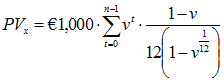
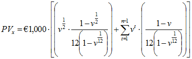
Life Annuity to Retiree
![]()
![]()
Note that this can also be expressed as:
![]()
Life Annuity to Active Member Decrementing due to Disability
In German mode, disability and death decrements are assumed to occur in the middle of the year. The annuities arising from these decrements therefore start in the middle of the year, and this mid-year commencement is reflected differently depending on the biometric formulae selected.
Biometric formulae 1998, 2005, and 2018
For these sets of formulae, the mid-year commencement is reflected through the payment frequency adjustment. Payments in the amount of k(m) times the annual benefit are treated as payable in the year of decrement.
![]()
Note that this can also be expressed as:
![]()
Death benefits (which are payable to a spouse) are valued in the same way, but spouse mortality is substituted for member mortality in the formulas above.
Biometric formulae 1983
For these formulae, the mid-year commencement is reflected through averaging beginning-of-year and end-of-year annuities.

where:

n Year Certain Annuity to Retiree
n Year Certain Annuity to Active Member Decrementing due to Disability
Because disability and death benefits are assumed to occur in the middle of the year, the annuities resulting from these benefits are assumed to commence in the middle of the year and this fact is reflected in the payment frequency adjustments. The adjustment in the year of decrement reflects payment for the last half of the year, whereas the adjustment in remaining years reflects payment for a full year.
50% J&S to Retiree, with Beneficiary Determined at Member Death
This is the sum of the values of a life annuity to the member (PVx below) and the entitlement to a surviving spouse’s pension (PVy(x) below). Because the beneficiary is determined at member death using actuarial assumptions, this is also known as the “collective method”. Surviving spouse annuities are assumed to commence, on average, in the middle of the year. In this example, we assume that the Joint and Survivor fractions entered in the payment form definition are 1 when only the member is alive and 0.5 when only the beneficiary is alive.

in which:
![]()
and the spouse present value depends on the biometric formulae, as follows:
Biometric formulae 1998, 2005, and 2018

where:
![]() is the probability of the member being married at death age x+t
is the probability of the member being married at death age x+t
![]()
Note that:
![]()
Biometric formulae 1983

where:

50% J&S to Active Member Decrementing due to Disability, with Beneficiary Determined at Member Death (or when using the Individual Method)
This is the sum of the values of a life annuity to the member (PVx below) and the entitlement to a surviving spouse’s pension (PVy(x) below). Because the beneficiary is determined at member death using actuarial assumptions, this is also known as the “collective method”. Disability decrement from active status is assumed to occur, on average, in the middle of the year. Surviving spouse annuities are also generally assumed to occur in the middle of the year. For death in the same year as decrement, however, the proportion of the year the spouse must survive depends on the Biometric Formulae option selected in the Decrements topic of Valuation Assumptions. For RT 2005/2018 the spouse must survive 1/2 of the year, for RT 1998 the spouse must survive 1/3 of the year, and for RT 1983 there is no spouse mortality applied in the year. In addition, the method of calculating the mid-year annuity value differs between RT 1983 and the other methods, in a way that is analigous to the J&S formula for a retiree above. For more details, see Payment form values for mid-year benefits.
Here we illustrate the RT 2005 methodology. In this example, we assume that the joint and survivor fractions entered in the payment form definition are 1 when only the member is alive and 0.5 when only the beneficiary is alive.
![]()
in which:
![]()
![]()
where:
![]() is the probability of the member being married at death age x+t
is the probability of the member being married at death age x+t
![]()
Note that:
![]()
If the Individual Method applies, then

where  and
and  represent the spouse mortality using the retiree and beneficiary mortality tables, respectively.
Life Insurance to Retiree
Life Insurance is always assumed to be paid at the end of the payment period. This example assumes that the life insurance is payable to all members upon death. If you deselect the option that life insurance is payable only to a surviving spouse, the factor of h below (i.e., the fraction married at the time of death) would be removed.
![]()
Thus
![]()
Summary for biometric formulae 1998, 2005, and 2018
In summary, payment frequency adjustments are calculated as follows:
| Death/Disability | Retirement | |||
| Beginning-of-Period | Life Contingent | Decrement Year | ||
| After Decrement Year | ||||
| Certain | Decrement Year |  (or 1/2 if v = 1) (or 1/2 if v = 1) |
 (or 1 if v = 1) (or 1 if v = 1) |
|
| After Decrement Year |  (or 1 if v = 1) (or 1 if v = 1) |
|||
| End-of-Period | Life Contingent | Decrement Year | ||
| After Decrement Year | ||||
| Certain | Decrement Year | 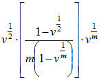 (or 1/2 if v = 1) (or 1/2 if v = 1) |
 (or 1 if v = 1) (or 1 if v = 1) |
|
| After Decrement Year | 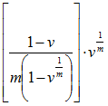 (or 1 if v = 1) (or 1 if v = 1) |